High-Resolution Color Image Deblurring
This tutorial walks through a complete example of the benchmark using the High-Resolution Color Image dataset. We will explore the dataset, configuration, and interpretation of results.
The Dataset: High-Resolution Color Image
What is it?
The high-resolution color image dataset is a multi-operator inverse problem where the goal is to recover a sharp color image from multiple blurred measurements. Each measurement is the original image degraded by a different anisotropic (directional) Gaussian blur.
Real-world analogy: Imagine taking photos of the same scene through different blurred lenses. Each photo is degraded differently. The goal is to recover the original sharp image using information from all these blurred observations.
Dataset Preview
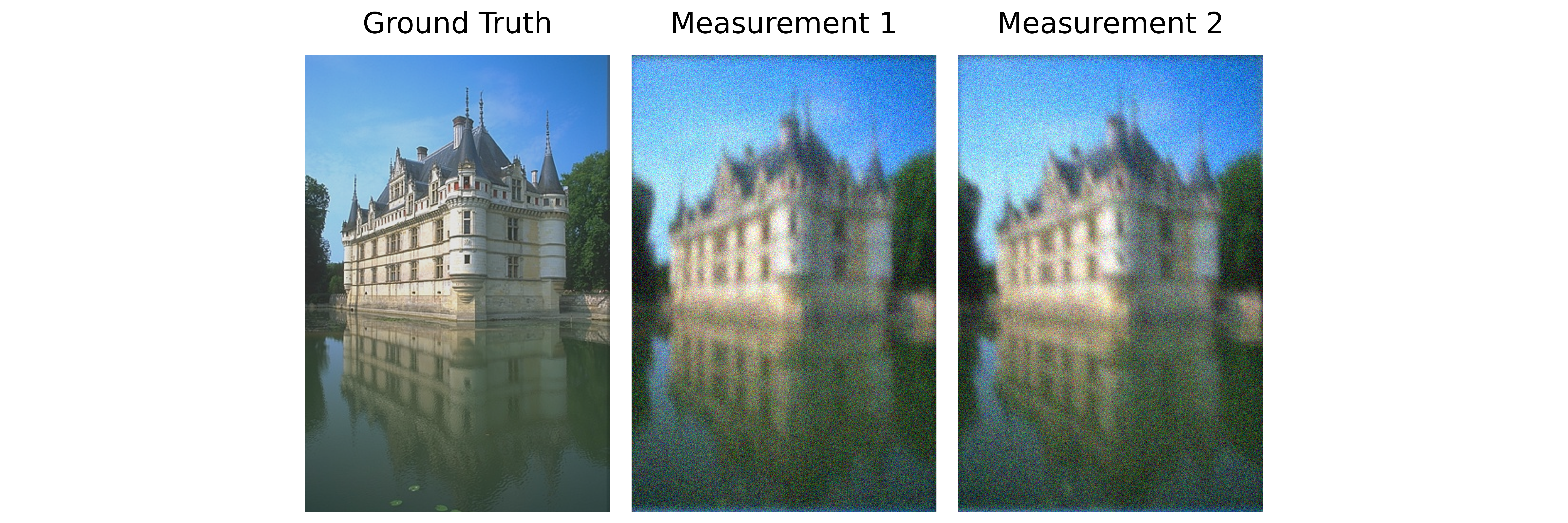
Left to right: Ground truth (original sharp image), Measurement 1 (blur angle 0°), Measurement 2 (blur angle 25.7°)
Configuration: Experiment Setup
Benchmark Purpose
This is a toy example designed to test distributed computing efficiency on large-scale inverse problems. The high-resolution image (2048×1366) combined with forward operators (8 blurs) and a pretrained prior (DRUNet) creates computational demands that benefit from distributed processing across multiple GPUs.
We use the configuration file configs/highres_imaging.yml to set up the experiment. The configuration specifies:
Objective: What metric to evaluate (PSNR, etc.)
Dataset: Which dataset to use and its parameters
Solver: Which solver to run and its hyperparameters
Execution Grid: Different GPU configurations to benchmark and compare
Execution Grid
The execution grid specifies different GPU configurations:
slurm_gres, slurm_ntasks_per_node, slurm_nodes, distribute_physics, distribute_denoiser, patch_size, overlap, max_batch_size: [
  ["gpu:1", 1, 1, false, false, 0, 0, 0],
  ["gpu:2", 2, 1, true, true, 448, 32, 0],
  ["gpu:4", 4, 1, true, true, 448, 32, 0],
  ]
Important: To ensure proper distributed parallelization, the number of tasks per node (slurm_ntasks_per_node) must equal the number of GPUs (slurm_gres). This ensures one process per GPU.
This creates a grid comparing three configurations:
Configuration 1: Single GPU (baseline)
["gpu:1", 1, 1, false, false, 0, 0, 0]
slurm_gres: gpu:1= 1 GPUslurm_ntasks_per_node: 1= 1 process per GPUdistribute_physics: false= No parallelization of blur operatorsdistribute_denoiser: false= Full image processed at oncePurpose: Baseline performance on limited resources
Configuration 2: 2-GPU with Distribution
["gpu:2", 2, 1, true, true, 448, 32, 0]
slurm_gres: gpu:2= 2 GPUsslurm_ntasks_per_node: 2= 2 processes (one per GPU)distribute_physics: true= Split 8 blur operators across 2 GPUs (4 each)distribute_denoiser: true= Spatial tiling: Split large image into patchespatch_size: 448= Each patch is 448×448 pixelsoverlap: 32= Overlap region for smooth transitions between patchesPurpose: Multi-GPU scalability with operator and spatial distribution
Configuration 3: 4-GPU with Increased Distribution
["gpu:4", 4, 1, true, true, 448, 32, 0]
Similar to Config 2, but with 4 GPUs.
Purpose: Further scalability test with more GPU resources
For more details on distributed computing, see the DeepInv distributed documentation.
Dataset Parameters
The dataset section configures the high-resolution color image problem:
dataset:
  - highres_color_image:
      image_size: 2048
      num_operators: 8
      noise_level: 0.1
Parameter Meanings:
image_size: The maximum dimension of the image.2048: Large (tests scalability on GPUs)num_operators: Number of different blur operators applied to create measurements.8: 8 measurements with different blur angles from 0° to 180°noise_level: Gaussian noise added to the measurements (in pixel intensity 0-1 range).0.1: Realistic noise (10% noise)
Solver
The solver section configures the Plug-and-Play (PnP) reconstruction algorithm:
solver:
  - PnP:
      denoiser: drunet
      denoiser_sigma: 0.005
      step_size: 0.1
      init_method: ["zeros"]
Solver Parameters:
denoiser: The pretrained denoiser to use as a prior.denoiser_sigma: Noise level hint passed to the denoiser. Helps the denoiser adapt to the noise level.step_size: Gradient descent step size. Controls convergence speed and stability.init_method: How to initialize the reconstruction.
Interpreting Results
Benchmark Results
Below is an interactive dashboard comparing the three configurations:
Interpretation
PSNR vs. Iteration & PSNR vs. Computation Time
All setups reach about the same final PSNR, so using multiple GPUs does not reduce reconstruction quality. The multi-GPU runs reach the target PSNR much faster than the single-GPU baseline, which shows the speedup clearly.
Time Breakdown: Gradient and Denoiser
The denoiser dominates runtime and is the main bottleneck. Adding more GPUs reduces denoiser time, but gradient time stays almost the same since the gradient step is cheap, and communication between GPUs often takes longer than the computation itself.
GPU Memory Usage: Gradient and Denoiser
For multi-GPU configurations, the max memory shown corresponds to rank 0 (the main process), which is similar to other ranks. Interestingly, the 2-GPU setup uses more denoiser memory (4.3 GB) than a single GPU (1.6 GB), because peak memory for some denoisers is highly sensitive to image dimensions, even with small changes in input size. See the takeaways page for more details.